Tutorials
Tomographic reconstructions
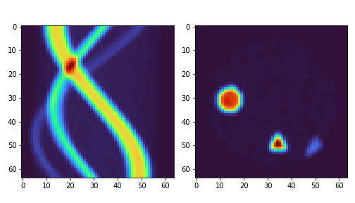
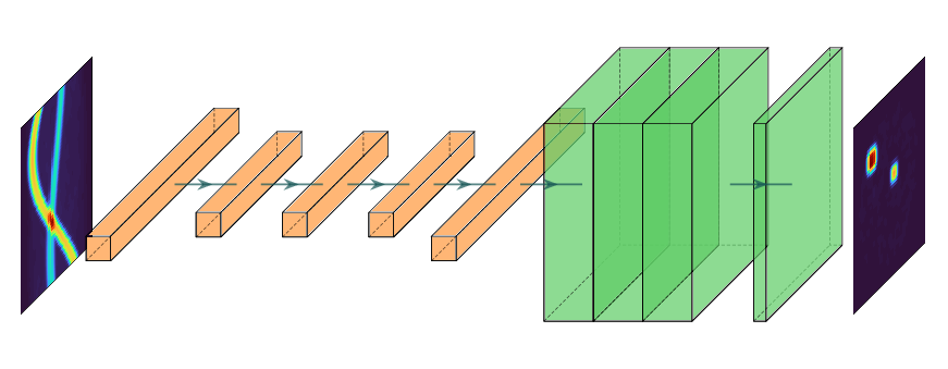
Reconstruction with a CNN
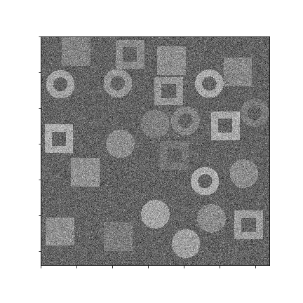
In this tutorial we will reconstruct an image from a sinogram using a convolutional neural network. We have a network architecture for this task: models.cnn_reconstruct.models.reconstruct_cnn
Step 0
Generate the data. We have some scripts to generate sample data for this task. LibShapes.py Alternatively download sample data from here: http://tiny.cc/vdl9rz
Step 1
When the data is generated we now load it up. Use the utils.tools.read_reconstruct_library helper function to make this easier. We then shuffle around the image/sinogram pairs to make sure that we don’t have any false ordering. We alsoe need to make sure that superres-ml is on our pythonpath. Split the data into training and test data.
import sys
sys.path.append('/path/to/super-resolution-ml/')
from utils.tools import read_reconstruct_library

images, sinos, nim = read_reconstruct_library('data/reconstruction/shapes_random_noise_64px_norm.h5')
index = np.arange(nim)
np.random.shuffle(index)
images = images[index,:,:,:]
sinograms = sinos[index,:,:,:]
sinograms_test = sinograms[9000:]
images_test = images[9000:]
sinograms = sinograms[:9000]
images = images[:9000]
Step 2
Set up the network. We import the reconstruct_cnn netowrk from out superres-ml model library. We then compile the network to use the Adam optimiser and to monitor the mae and mse during training. We add a callback, which makes the training stop if the metrics have not improved for three steps.
from tensorflow.keras.optimizers import Adam
from tensorflow.keras.callbacks import EarlyStopping
from models.cnn_reconstruct.models import reconstruct_cnn

model_rec = reconstruct_cnn(sinos.shape[1], sinos.shape[2])
model_rec.compile(optimizer = Adam(lr = 0.000025), loss = 'mean_squared_error', metrics = ['mae', 'mse'])
my_callbacks = [EarlyStopping(patience=3)]
Step 3
Train the model!
training = model_rec.fit(sinograms, images,
                      validation_split = 0.1,
                      batch_size=32,
                      epochs = 100,
                      verbose = True,
                      callbacks=my_callbacks)
history = model_rec.history
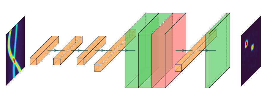
Reconstruction with a Dense Network
This tutorial is just like the one above, but we use a dense network at the start before convolutions. This kind of network gives very good results but requires huge memory for any larger images. See the architecture below.
Steps 0, 1 and 3 are the exact same as for the CNN.
Step 0
Generate the data. We have some scripts to generate sample data for this task. LibShapes.py Alternatively download sample data from here: http://tiny.cc/vdl9rz
Step 1
When the data is generated we now load it up. Use the utils.tools.read_reconstruct_library helper function to make this easier. We then shuffle around the image/sinogram pairs to make sure that we don’t have any false ordering. We alsoe need to make sure that superres-ml is on our pythonpath. Split the data into training and test data.
from utils.tools import read_reconstruct_library
import sys
sys.path.append('/path/to/super-resolution-ml/')

images, sinos, nim = read_reconstruct_library('data/reconstruction/shapes_random_noise_64px_norm.h5')
index = np.arange(nim)
np.random.shuffle(index)
images = images[index,:,:,:]
sinograms = sinos[index,:,:,:]
sinograms_test = sinograms[9000:]
images_test = images[9000:]
sinograms = sinograms[:9000]
images = images[:9000]
Step 2
Set up the network. We import the reconstruct_cnn netowrk from out superres-ml model library. We then compile the network to use the Adam optimiser and to monitor the mae and mse during training. We add a callback, which makes the training stop if the metrics have not improved for three steps.
from tensorflow.keras.optimizers import Adam
from tensorflow.keras.callbacks import EarlyStopping
from models.dense_reconstruct.models import dense_reconstruct

model_rec = dense_reconstruct(sinos.shape[1], sinos.shape[2])
model_rec.compile(optimizer = Adam(lr = 0.000025), loss = 'mean_squared_error', metrics = ['mae', 'mse'])
my_callbacks = [EarlyStopping(patience=3)]
Step 3
Train the model!
training = model_rec.fit(sinograms, images,
                      validation_split = 0.1,
                      batch_size=32,
                      epochs = 100,
                      verbose = True,
                      callbacks=my_callbacks)
history = model_rec.history
Reconstruction with a Automap
This tutorial is just like the one above, but we use a dense network at the start before convolutions. This kind of network gives very good results but requires huge memory for any larger images. See the architecture below.
Steps 0, 1 and 3 are the exact same as for the CNN and dense architectures.
Step 0
Generate the data. We have some scripts to generate sample data for this task. LibShapes.py Alternatively download sample data from here: http://tiny.cc/vdl9rz
Step 1
When the data is generated we now load it up. Use the utils.tools.read_reconstruct_library helper function to make this easier. We then shuffle around the image/sinogram pairs to make sure that we don’t have any false ordering. We alsoe need to make sure that superres-ml is on our pythonpath. Split the data into training and test data.
from utils.tools import read_reconstruct_library
import sys
sys.path.append('/path/to/super-resolution-ml/')

images, sinos, nim = read_reconstruct_library('data/reconstruction/shapes_random_noise_64px_norm.h5')
index = np.arange(nim)
np.random.shuffle(index)
images = images[index,:,:,:]
sinograms = sinos[index,:,:,:]
sinograms_test = sinograms[9000:]
images_test = images[9000:]
sinograms = sinograms[:9000]
images = images[:9000]
Step 2
Set up the network. We import the reconstruct_cnn netowrk from out superres-ml model library. We then compile the network to use the Adam optimiser and to monitor the mae and mse during training. We add a callback, which makes the training stop if the metrics have not improved for three steps.
from tensorflow.keras.optimizers import Adam
from tensorflow.keras.callbacks import EarlyStopping
from models.automap.models import automap

model_rec = automap(sinos.shape[1], sinos.shape[2])
model_rec.compile(optimizer = Adam(lr = 0.000025), loss = 'mean_squared_error', metrics = ['mae', 'mse'])
my_callbacks = [EarlyStopping(patience=3)]
Step 3
Train the model!
training = model_rec.fit(sinograms, images,
                      validation_split = 0.1,
                      batch_size=32,
                      epochs = 100,
                      verbose = True,
                      callbacks=my_callbacks)
history = model_rec.history
Segmentation of X-ray images
Binary segmentation
This tutorial looks at segmentation of sections of an image, for example collected from X-ray imaging. We have a set of images where we have already labelled what the different parts of the image are, now we want to train and apply a model to another set, labelling new X-ray images.
To do this we will use a U-net architecture. There is one big challenge in using most U-net architectures that you will find on the web.
The image sizes are very large. This means that the image and the model cannot fit together in the memory.
To overcome the problem we will use a routine in superres-tomo to create patches from the image and learn sequentially from each patch. To do do this we have implemented the data_handeling.generators.mask_patch_from_file function which acts as a generator to feed the network for training.
Step 0
Generate the data. There is a helper script in the directory data/segmentation run this to generate the data for this tutorial. Run this script to generate the data for this tutorial.
Also make sure the superres-ml package is in your pythonpath
import sys
sys.path.append('/path/to/super-resolution-ml/')
Step 1
Once the data is in place we are ready to start setting up the U-net. Tell the code where to find the images and masks, the types of file to expect.
datapath= 'data/segmentation/train/' #<the root directory of images and masks for training>
valpath= 'data/segmentation/val/' #<the root directory of images and masks for validation>
img_dir= 'noiseless/' # <the subdirectory where images are>
mask_dir= 'label/' #<the subdirectory where masks are>
ftypes= ['./tiff'] # (<filetypes to look for>) # e.g. ('.tif')
Step 2
Set up the information about the size of the original image and the size of the patches to take from the image. Also here you can define a list of which patches to use. This last feature is useful when the interesting features are only in a section of the image. You can specify the particular patches to consider for the training. The numbering of patches starts from zero and proceeds left to right top to bottom. If the patch list is left empty the generator uses all patches.
image_shape = (1280, 1280)
patch_shape = (64, 64)
patch_range = []
Step 3
Set up the generator. This is the function that will flow the patches from the images to the netowrk for training.
from data_handeling.generators import mask_patch_from_file

myGene = mask_patch_from_file(datapath,
                           img_dir, mask_dir,
                           patch_shape, image_shape,
                           types = ftypes, patch_range=patch_range,
                           debug=False,
                           batch_size = 1,
                           normalise_images=False)

valGene = mask_patch_from_file(valpath,
                        img_dir, mask_dir,
                        patch_shape, image_shape,
                        types = ftypes, patch_range=patch_range,
                        debug=False,
                        batch_size = 1,
                        normalise_images=False)
Step 4
Define the netowrk architecture, the hyperparameters and the training time. Here the input size is the dimension of the patches, also we have just 1 channel as the image is greyscale. We use a standard Adam optimiser. We use binary_crossentropy as the loss function and also monitor the accuracy during training.
from models.u_net.models import unet_3layer
import models.losses.custom_loss_functions as losses
from tensorflow.keras.optimizers import Adam

model = unet_3layer(input_size = (patch_shape[0], patch_shape[1], 1))
opt = Adam()
model.compile(loss=losses.weighted_cross_entropy(2), optimizer=opt,
           metrics=["accuracy"])
Step 5
Train and save!
epochs = 6
steps_per_epoch = 2000
model.fit(myGene, steps_per_epoch=steps_per_epoch,
          epochs=epochs, validation_data=valGene, validation_steps=100)
model.save_weights('saved_weights.hdf5')
Step 6
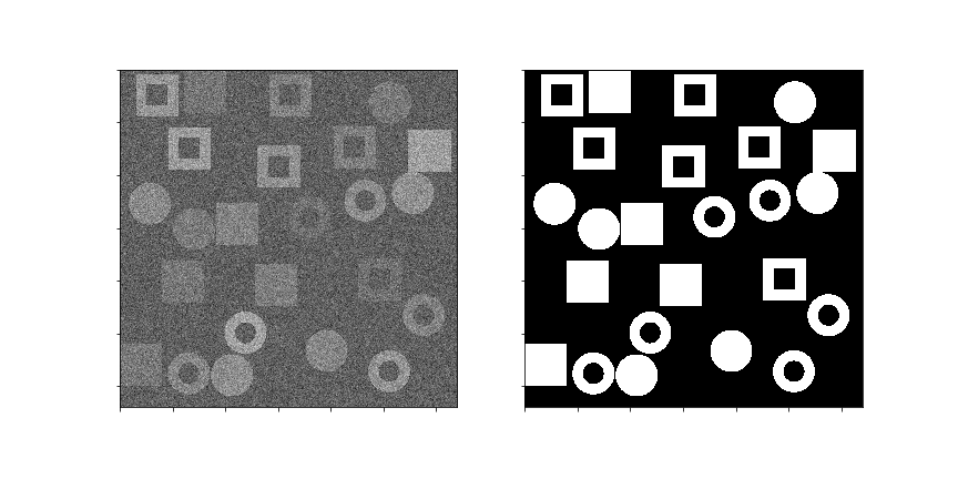
Run the model for inference. Having trained the model on some images you can now try to deploy on
new examples. We have the utils.tools.inference_binary_segmentation() helper
function to do this. First we load up the saved model and weights.
from  utils.tools import inference_binary_segmentation

datapath = 'data/segmentation/test/noiseless/'
patch_shape = (64, 64)
image_shape = (1280, 1280)
savepath = './inferred_masks/'

inference_binary_segmentation(datapath, patch_shape, image_shape, model,
              file_prefix='binary_mask', savepath=savepath, fig_size=(8, 8),
             normim=False)
In the inferred_masks directory there should now be a masking file something like:
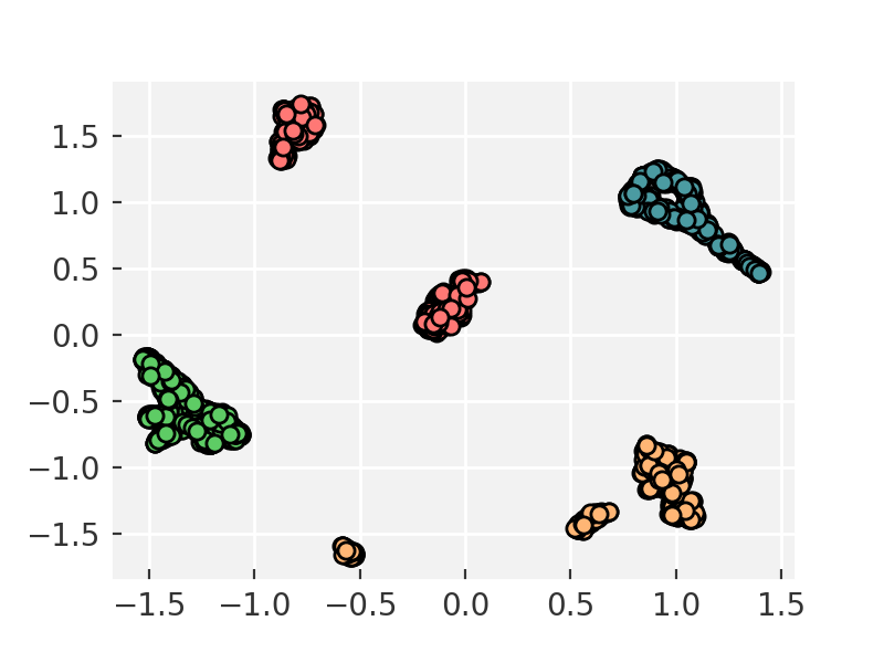
Dimension reduction
This module allows one to project a dataset of images into lower dimensional space (2 or 3 D usually). It is very useful for inspeting datasets to look for outliers and anomallies. It is also useful to see if a new image is out of the training distribution, which can be a problem for CNN based reconstructions. See our paper Identifying and avoiding training set bias in neural networks for tomographic image reconstruction for a discussion of this.
If you do not already have the data you can download it from
- Sinograms: https://tinyurl.com/y2t56hgd
- Images: https://tinyurl.com/y2l4jvoj
Then unzip the data. It contains datasets used in our paper. In the example below we load 2000 sinograms, taken from all of the materials.
import sys
sys.path.append('/path/to/super-resolution-ml/')
from utils.tools import read_reconstruct_library

images, sinos, nim = read_reconstruct_library('./All_mixed_2K_sinograms_raw.h5')
Run the dimensionality reduction. The code below will convert each of your images to a 2D vector. You can alter the settings of the dimensionality reduction. The code uses the scikit-learn implementation of tSNE to reduce dimensions. You can change the number of desired output dimensions by passing the n_components_tsne to the function, by default it is 2.
x = dimension_reducer(sinos)
Plot and inspect your result. You can now look at the reduced dimesnion map to see if there are any outliers or anomalies.
plt.scatter(x[:, 0], x[:, 1])
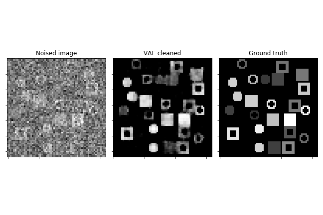
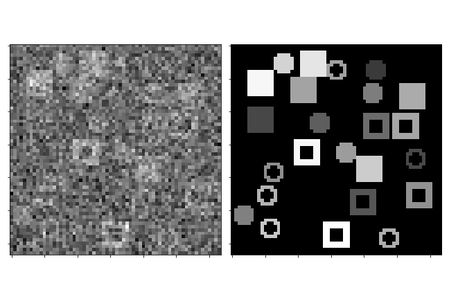
Denoising of X-ray images
Variational Autoencoder
Often images that are reconstructed contain low signal to noise ratios, if the dose was low or the collection time short. In these cases it would often be desireable to remove the noise and accentuate the signal in an image. We can do this using a Variational Autoencoder (VAE)
Step 0
Set up the data. You can use the data/denoising/generatedata.py script to generate some example data. Then use the helper functions build_list_images and build_autoencoder_data to build the data set ready to train the VAE.
We need to specify the data shape with the input_data keyword and then specify directories to find the training and validation inputs and labels.
import sys
sys.path.append('/path/to/super-resolution-ml/')
from data_handeling.tools import build_list_images
from models.autoencoder.tools import build_autoencoder_data

input_data = (64, 64, 1)

datapath = '../data/denoising/train/noisy/'
Xfiles = build_list_images(datapath, types = ['.tiff'])
datapath = '../data/denoising/train/noiseless/'
yfiles = build_list_images(datapath, types = ['.tiff'])
X, labels = build_autoencoder_data(Xfiles, yfiles=yfiles, input_data=input_data)
datapath = '../data/denoising/test/noisy/'
Xfiles = build_list_images(datapath, types = ['.tiff'])
datapath = '../data/denoising/test/noiseless/'
yfiles = build_list_images(datapath, types = ['.tiff'])
xtest, ltest = build_autoencoder_data(Xfiles, yfiles, input_data=input_data)
Step 1
Set up the VAE. Here we import the model as well as functions to train and run the model and an optimiser. We need to set the number of units to use in the bottle-neck (latent) space.
from models.autoencoder.models import CVAE
from models.autoencoder.tools import vae_train, vae_inference
from tensorflow.keras.optimizers import Adam

latent_dim = 16
optimizer = Adam(lr=0.0001)
epochs = 500
model = CVAE(latent_dim, input_data)
Step 2
Train the model. Using the vae_train function set the model to train.
vae_train(model, X, labels, xtest, ltest, epochs, optimizer, sigmoid=False)
Step 3
Try the trained model out on some of the test data.
out = vae_inference(model, np.expand_dims(X[9], axis=0), sigmoid=True)